TASK 2.1: Visualize quantum circuits
- Which parameter of the
draw()method specifies the output format of the quantum circuit visualization?
a. style
b. output
c. format
d. backend
answer
The answer is b.
The QuantumCircuit.draw() method uses the parameter output to specify the format of the visualization. Options include "text" (ASCII art), "mpl" (Matplotlib), "latex", and "latex_source".
from qiskit import QuantumCircuit
from qiskit.visualization import circuit_drawer
qc = QuantumCircuit(1, 1)
qc.h(0)
qc.measure(0, 0)
qc.draw(output="mpl")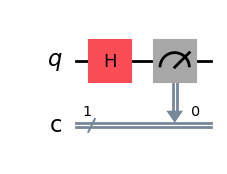
- When calling
circuit.draw(output="mpl"), what backend is used to generate the visualization?
a. ASCII art
b. Matplotlib
c. Text drawer
d. LaTeX
answer
The answer is b.
When using circuit.draw(output="mpl"), the Matplotlib backend is called to render the circuit as a figure. Other options include "text" for ASCII drawings and "latex" for LaTeX rendering.
- Given the following code:
from qiskit import QuantumCircuit

qc = QuantumCircuit(2)
qc.h(0)
qc.cx(0, 1)
qc.measure_all()

qc.draw(output="text")
Which of the following diagrams best matches the output?
a.
        ┌───┐      ░ ┌─┐
   q_0: ┤ H ├──■───░─┤M├───
        └───┘┌─┴─┐ ░ └╥┘┌─┐
   q_1: ─────┤ X ├─░──╫─┤M├
             └───┘ ░  ║ └╥┘
meas: 2/══════════════╩══╩═
                      0  1
b.
             ┌───┐ ░ ┌─┐
   q_0: ──■──┤ H ├─░─┤M├───
        ┌─┴─┐└───┘ ░ └╥┘┌─┐
   q_1: ┤ X ├──────░──╫─┤M├
        └───┘      ░  ║ └╥┘
meas: 2/══════════════╩══╩═
                      0  1
c.
        ┌───┐┌───┐ ░ ┌─┐
   q_0: ┤ X ├┤ H ├─░─┤M├───
        └─┬─┘└───┘ ░ └╥┘┌─┐
   q_1: ──■────────░──╫─┤M├
                   ░  ║ └╥┘
meas: 2/══════════════╩══╩═
                      0  1
d.
        ┌───┐ ░ ┌─┐
   q_0: ┤ H ├─░─┤M├───
        ├───┤ ░ └╥┘┌─┐
   q_1: ┤ X ├─░──╫─┤M├
        └───┘ ░  ║ └╥┘
meas: 2/═════════╩══╩═
                 0  1
answer
The answer is a.
The circuit applies an H gate on qubit 0, then a CX gate from qubit 0 to qubit 1, followed by measurement of both qubits. This matches the diagram with H on q0, CX connecting q0 → q1, and measurements on both qubits.
TASK 2.2: Visualize quantum measurements
- Which function should you use to visualize measurement outcome counts from a circuit or sampler result?
a. plot_state_qsphere
b. plot_histogram
c. plot_state_city
d. plot_bloch_vector
answer
The answer is b.
Use plot_histogram from qiskit.visualization to visualize measurement result counts (bitstrings and their frequencies). This is the canonical way to visualize quantum measurement outcomes, as opposed to state visualizers like qsphere or Bloch charts which depict state amplitudes or vectors rather than sampled counts.
from qiskit.visualization import plot_histogram

counts1 = {'00': 499, '11': 501}
counts2 = {'00': 511, '11': 489}

data = [counts1, counts2]
plot_histogram(data)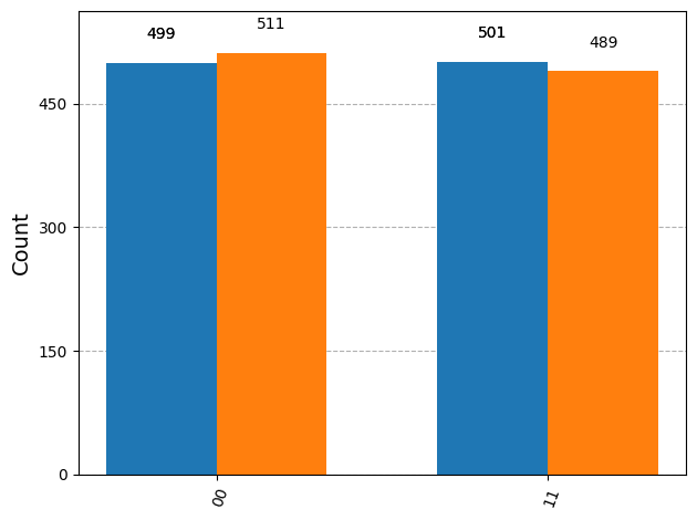
- You obtained a
Statevectorand want a measurement-like distribution to plot without running on hardware. Which API produces shot-based counts that you can pass toplot_histogram?
a. state.draw_counts(shots=1024)
b. state.sample_counts(shots=1024)
c. state.measure_all(shots=1024)
d. state.to_counts(shots=1024)
answer
The answer is b.
Statevector.sample_counts(shots=...) samples from the state’s probability distribution and returns a counts dictionary compatible with plot_histogram, letting you visualize expected measurement outcomes without executing on a backend.
- In dynamic circuits, which builder creates a conditional block that has only a True branch (no explicit else branch), typically used for mid-circuit measurement feedforward?
a. QuantumCircuit.if_else
b. QuantumCircuit.switch
c. QuantumCircuit.if_test
d. QuantumCircuit.c_if
answer
The answer is c.
if_test builds a control-flow region with a True body only, perfect when you want to apply operations conditionally on a classical-bit outcome from a mid-circuit measurement. if_else includes both True and False bodies; c_if is legacy-style conditional execution tied to instruction conditions.
- Which code fragment correctly measures
q0intoc0mid-circuit and appliesx(q1)only when the measurement outcome is 1, before the final measurement ofq1?
a.
qc.measure(0, 0)
qc.if_test((qc.clbits[0], 1)):
    qc.x(1)
qc.measure(1, 1)
b.
qc.measure(0, 0)
with qc.if_test((qc.clbits[0], 1)):
    qc.x(1)
qc.measure(1, 1)
c.
with qc.if_test((qc.clbits[0], 1)):
    qc.measure(0, 0)
    qc.x(1)
qc.measure(1, 1)
d.
with qc.if_else((qc.clbits[0], 1)) as else_:
    qc.x(1)
with else_:
    pass
qc.measure([0,1], [0,1])
answer
The answer is b.
The measurement of q0 must occur before the if_test so its outcome populates c0. The context-manager form with qc.if_test((cbit, 1)): introduces a True-only region; x(1) executes only when the condition is met. Options a/d don’t use the context-manager correctly, and c measures inside the conditional (so the condition wouldn’t be defined when entering the block).
- When plotting measurement histograms for multiple executions on the same axes, which keyword argument helps distinguish them in the legend?
a. title=['run A', 'run B']
b. labels=['run A', 'run B']
c. legend=['run A', 'run B']
d. caption=['run A', 'run B']
answer
The answer is c.
Pass legend=[...] to plot_histogram when plotting multiple result sets in one chart so each set of bars is labeled (e.g., comparing ideal vs. noisy counts).
plot_histogram(data, legend=['run A', 'run B'])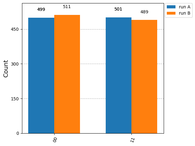
- You have a large number of possible bitstrings in the measurement outcomes and want the histogram to show only the top 8, aggregating the rest in a single bar. Which option should you set?
a. bins=8
b. truncate=8
c. max_terms=8
d. number_to_keep=8
answer
The answer is d.
number_to_keep limits how many terms are displayed; the remaining outcomes are grouped into a bar labeled “rest,” keeping the measurement visualization readable.
- To sort histogram bars by their counts from highest to lowest (useful for quickly spotting dominant measurement outcomes), which argument should you use?
a. sort='desc'
b. order='descending'
c. sorted=True
d. rank='top'
answer
The answer is a.
Use sort='desc' (or 'asc') with plot_histogram to control bar ordering by counts, which helps interpret noisy vs. ideal measurement distributions.
- In a circuit diagram that uses mid-circuit measurement with dynamic control flow, how is the measurement information visualized?
a. The diagram suppresses classical wires; measurement effects are implicit.
b. Measurements draw arrows from qubit wires to classical clbit wires, and conditional regions (if_test, etc.) appear as boxed blocks that are annotated by the classical condition.
c. Measurements are drawn as statevector spheres; conditions are tagged on the spheres.
d. Measurements show only as labels on gates; there are no classical wires or conditional regions.
answer
The answer is b.
Qiskit’s circuit drawers render measurement ops with arrows from qubit to classical wires, then depict control-flow regions (e.g., if_test, if_else) as boxed/annotated blocks tied to the classical condition—making the path from measurement to conditional execution explicit in the visualization.
TASK 2.3: Visualize quantum states
- Which Qiskit visualization function can be used to compare measurement results of multiple experiments?
a. plot_histogram
b. plot_bloch_vector
c. plot_state_qsphere
d. plot_gate_map
answer
The answer is a.
The plot_histogram() function is designed to show measurement outcomes, and it can overlay results from multiple experiments, making it suitable for comparison.
plot_histogram(data)from math import pi
from qiskit import QuantumCircuit
from qiskit.quantum_info import Statevector
from qiskit.visualization import plot_bloch_multivector
# Create a Bell state for demonstration
qc = QuantumCircuit(2)
qc.h(0)
qc.crx(pi / 2, 0, 1)
psi = Statevector(qc)
plot_bloch_multivector(psi)
# Alternative: psi.draw("bloch")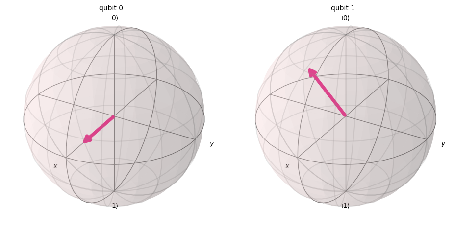
from qiskit.visualization import plot_state_qsphere

plot_state_qsphere(psi)
# Alternative: psi.draw("qsphere")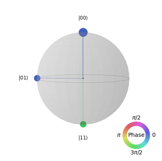
from qiskit.providers.fake_provider import GenericBackendV2
from qiskit.visualization import plot_gate_map

backend = GenericBackendV2(num_qubits=5)

plot_gate_map(backend)
---------------------------------------------------------------------------
MissingOptionalLibraryError Traceback (most recent call last)
Cell In[7], line 6
2 from qiskit.visualization import plot_gate_map
4 backend = GenericBackendV2(num_qubits=5)
----> 6 plot_gate_map(backend)
File ~/work/qiskit-certification-prep/qiskit-certification-prep/.venv/lib/python3.11/site-packages/qiskit/utils/lazy_tester.py:165, in LazyDependencyManager.require_in_call.<locals>.out(*args, **kwargs)
162 @functools.wraps(function)
163 def out(*args, **kwargs):
164 self.require_now(feature)
--> 165 return function(*args, **kwargs)
File ~/work/qiskit-certification-prep/qiskit-certification-prep/.venv/lib/python3.11/site-packages/qiskit/visualization/gate_map.py:918, in plot_gate_map(backend, figsize, plot_directed, label_qubits, qubit_size, line_width, font_size, qubit_color, qubit_labels, line_color, font_color, ax, filename, qubit_coordinates)
913 if len(qubit_coordinates) != num_qubits:
914 raise QiskitError(
915 f"The number of specified qubit coordinates {len(qubit_coordinates)} "
916 f"does not match the device number of qubits: {num_qubits}"
917 )
--> 918 return plot_coupling_map(
919 num_qubits,
920 qubit_coordinates,
921 coupling_map.get_edges(),
922 figsize,
923 plot_directed,
924 label_qubits,
925 qubit_size,
926 line_width,
927 font_size,
928 qubit_color,
929 qubit_labels,
930 line_color,
931 font_color,
932 ax,
933 filename,
934 planar=rx.is_planar(coupling_map.graph.to_undirected(multigraph=False)),
935 )
File ~/work/qiskit-certification-prep/qiskit-certification-prep/.venv/lib/python3.11/site-packages/qiskit/utils/lazy_tester.py:165, in LazyDependencyManager.require_in_call.<locals>.out(*args, **kwargs)
162 @functools.wraps(function)
163 def out(*args, **kwargs):
164 self.require_now(feature)
--> 165 return function(*args, **kwargs)
File ~/work/qiskit-certification-prep/qiskit-certification-prep/.venv/lib/python3.11/site-packages/qiskit/utils/lazy_tester.py:164, in LazyDependencyManager.require_in_call.<locals>.out(*args, **kwargs)
162 @functools.wraps(function)
163 def out(*args, **kwargs):
--> 164 self.require_now(feature)
165 return function(*args, **kwargs)
File ~/work/qiskit-certification-prep/qiskit-certification-prep/.venv/lib/python3.11/site-packages/qiskit/utils/lazy_tester.py:221, in LazyDependencyManager.require_now(self, feature)
219 if self:
220 return
--> 221 raise MissingOptionalLibraryError(
222 libname=self._name, name=feature, pip_install=self._install, msg=self._msg
223 )
MissingOptionalLibraryError: "The 'Graphviz' library is required to use 'plot_coupling_map'. To install, follow the instructions at https://graphviz.org/download/. Qiskit needs the Graphviz binaries, which the 'graphviz' package on pip does not install. You must install the actual Graphviz software."- Which visualization method best shows the relative phase of each basis state in a quantum statevector?
a. plot_bloch_multivector
b. plot_state_qsphere
c. plot_histogram
d. circuit.draw(output="mpl")
answer
The answer is b.
The plot_state_qsphere() function shows the relative amplitudes and phases of quantum states on a sphere, making it the best choice for analyzing phase relationships.
- What does the function
plot_bloch_multivector()visualize?
a. Measurement outcomes as a bar chart
b. The density matrix as a heatmap
c. Each qubit’s state on the Bloch sphere
d. The connectivity of qubits on hardware
answer
The answer is c.
plot_bloch_multivector() displays each individual qubit’s state on the Bloch sphere. This allows visualization of single-qubit orientations within a multi-qubit quantum state.
- Which of the following visualizations explicitly requires a
StatevectororDensityMatrixobject as input?
a. plot_state_qsphere
b. plot_bloch_multivector
c. plot_state_city
d. All of the above
answer
The answer is d.
All three functions—plot_state_qsphere, plot_bloch_multivector, and plot_state_city—require a Statevector or DensityMatrix as input. They cannot operate directly on circuits without first computing the state.
- Which function displays the connectivity and coupling map of a quantum device?
a. plot_device_layout
b. plot_histogram
c. plot_gate_map
d. plot_coupling
answer
The answer is c.
plot_gate_map() visualizes the coupling map of a quantum device, showing qubit layout and connectivity. This is essential for understanding how two-qubit gates can be executed on real hardware.
from qiskit.providers.fake_provider import GenericBackendV2
from qiskit.visualization import plot_gate_map

backend = GenericBackendV2(num_qubits=5)

plot_gate_map(backend)- What additional argument can be passed to
plot_histogramto display multiple experiment results on the same chart?
a. merge=True
b. legend
c. compare=True
d. stacked=True
answer
The answer is b.
The legend argument in plot_histogram() allows labeling multiple experiment results when displayed on the same chart, making it easier to distinguish them.
- Which visualization tool can be used to see the real and imaginary components of a quantum state as a 3D bar chart?
a. plot_state_city
b. plot_histogram
c. plot_state_qsphere
d. plot_bloch_multivector
answer
The answer is a.
plot_state_city() represents the real and imaginary parts of a quantum state as 3D bar charts, providing an intuitive way to see amplitude contributions of each basis state.
from qiskit.visualization import plot_state_city

plot_state_city(psi)
# Alternative: psi.draw("city")- Given the following code:
from qiskit import QuantumCircuit
from qiskit.quantum_info import Statevector
from qiskit.visualization import plot_state_qsphere

qc = QuantumCircuit(2)
qc.h(0)
qc.cx(0, 1)
state = Statevector.from_instruction(qc)
plot_state_qsphere(state)
Which of the following best describes the qsphere output?
a. Two points at |00⟩ and |11⟩ with equal size, both colored the same.
b. Two points at |01⟩ and |10⟩ with equal size, opposite colors.
c. Four points at |00⟩, |01⟩, |10⟩, |11⟩ equally distributed.
d. A single point at |00⟩ only.
answer
The answer is a.
The circuit creates a Bell state (|00⟩ + |11⟩)/√2. On the qsphere, only |00⟩ and |11⟩ appear, both with equal amplitude and identical phase (same color).
from qiskit import QuantumCircuit
from qiskit.quantum_info import Statevector
from qiskit.visualization import plot_state_qsphere

qc = QuantumCircuit(2)
qc.h(0)
qc.cx(0, 1)
state = Statevector.from_instruction(qc)
plot_state_qsphere(state)- Given the following code:
from qiskit.quantum_info import Statevector
from qiskit.visualization import plot_bloch_multivector

state = Statevector([1/2, 1/2, 1/2, 1/2])
plot_bloch_multivector(state)
Which of the following describes the Bloch sphere plot?
a. Both qubits point along +X axis.
b. Both qubits point along +Z axis.
c. First qubit along +X, second along –X.
d. Random orientation with no symmetry.
answer
The answer is a.
The state [1/2, 1/2, 1/2, 1/2] corresponds to both qubits being in |+⟩ = (|0⟩ + |1⟩)/√2. On the Bloch sphere, |+⟩ points along the +X axis, so both qubits align in that direction.
from qiskit.quantum_info import Statevector
from qiskit.visualization import plot_bloch_multivector

state = Statevector([1/2, 1/2, 1/2, 1/2])
plot_bloch_multivector(state)- Given the code:
from qiskit import QuantumCircuit
from qiskit.quantum_info import Statevector
from qiskit.visualization import plot_state_city

qc = QuantumCircuit(1)
qc.h(0)
state = Statevector.from_instruction(qc)
plot_state_city(state)
Which of the following bar plots is expected?
a. Two tall bars at Re(|0⟩) and Re(|1⟩), equal height.
b. One tall bar at Re(|0⟩) only.
c. Two tall bars at Im(|0⟩) and Im(|1⟩).
d. Four bars with random heights.
answer
The answer is a.
Applying H to a single qubit creates (|0⟩ + |1⟩)/√2. In the state city plot, this results in two bars of equal height in the real part for |0⟩ and |1⟩, with no imaginary component.
from qiskit import QuantumCircuit
from qiskit.quantum_info import Statevector
from qiskit.visualization import plot_state_city

qc = QuantumCircuit(1)
qc.h(0)
state = Statevector.from_instruction(qc)
plot_state_city(state)